1 Kinetics 1.4 The velocity and speed distributions 1.6 Pressure and effusion

1.5 Change of variables and solid angles

(September 1, 2023)

1.5.1 Change of variables in 1d

Given a variable $x$ and its probability distribution

{\rm d}\mathscr{P}_{x}=P(x)\,{\rm d}x

(1.54)

How do we find the probability of $u$ , given a map $\varphi:x\rightarrow u$ , i.e. when $u(x)$ is a function of $x$ ? Assuming that that the map is one to one we have

{\rm d}\mathscr{P}_{u}=P(x(u))\left|\frac{dx}{du}\right|{\rm d}u=P(x(u))\frac{% {\rm d}u}{|\frac{du}{dx}|}

(1.55)

We note the absolute values here, which reflects the fact that when discussing probability we are asking whether a particle is in a bin of size ${\rm d}u$ , and the bin size isn’t like positive or negative.

The general formula for change of variables for an unoriented integral (like probability) is ³³ 3 The difference between oriented and unoriented integral is a matter of semantics at this level. If one replaces an integral by a sum of rectangles, you can sum them up in order from the beginning to the end (an oriented integral), or you can sum them up in any order provided they are in a specified region (an unoriented integral).

\int_{R}f(x){\rm d}x=\int_{R_{u}}f(x(u))\left|\frac{dx}{du}\right|\,{\rm d}u

(1.56)

Here $R$ is the region of integration for $x$ (for example $R$ could be interval $[1,2]$ ), and $R_{u}$ is the image of $R$ under the map (for example if the map is $u(x)=-2x$ then $R_{u}$ is $[-4,-2]$ ).

To set yourself straight of this notation just make the change of variables in a simple integral, getting the signs right. For example, consider the basic integral:

I=\int^{2}_{1}{\rm d}x=\int_{[1,2]}{\rm d}x=\frac{1}{2}

(1.57)

Undergoing a change of variables with $u=-2x$ , giving $x=-u/2$ and $dx=-\frac{1}{2}du$ , with $|dx/du|=\tfrac{1}{2}$ . The integral then becomes

I=\int^{-4}_{-2}\left(-\frac{1}{2}\right){\rm d}u=\int^{-2}_{-4}\frac{1}{2}{% \rm d}u=\int_{[-4,-2]}\,\frac{1}{2}\,{\rm d}u=1

(1.58)

1.5.2 Higher dimensions: spherical coordinates and solid angle

In higher-dimensions we have

{\rm d}\mathscr{P}=P(x,y,z)\,\underbrace{{\rm d}x\,{\rm d}y\,{\rm d}z}_{\mbox{% {\rm d}V}}

(1.59)

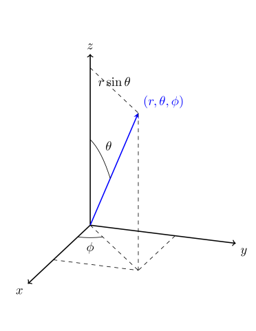
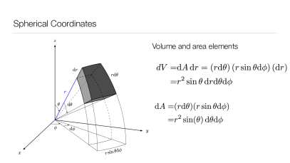
where ${\rm d}{V}$ is the “volume element”. We will use spherical coordinates $x=r\sin\theta\cos\phi$ , $y=r\sin\theta\sin\phi$ , and $z=r\cos\theta$ (see Fig. 1.1).

Figure 1.1: Spherical coordinates. Use the picture to justify $x=r\sin\theta\cos\phi$ , $y=r\sin\theta\sin\phi$ and $z=r\cos\theta$ .

A bit of geometry shows that the differential area $d A$ and the volume element $d V$ in spherical coordinates are (see Fig. 1.2)

	$\displaystyle dA=$	$\displaystyle r^{2}\sin\theta\,{\rm d}\theta\,{\rm d}\phi$		(1.60)
	$\displaystyle dV=$	$\displaystyle dA\,{\rm d}r=r^{2}\sin\theta\,{\rm d}r\,{\rm d}\theta\,{\rm d}\phi$		(1.61)

Figure 1.2: Spherical coordinates. From the figure, justify Eq. (1.60)

So in spherical coordinates

	$\displaystyle{\rm d}\mathscr{P}=$	$\displaystyle P(x,y,z)r^{2}\sin\theta\,{\rm d}r\,{\rm d}\theta\,{\rm d}\phi$		(1.62)
	$\displaystyle\equiv$	$\displaystyle P(r,\theta\,\phi){\rm d}r\,{\rm d}\theta\,{\rm d}\phi$		(1.63)

For example, if

P(x,y,z)=Ce^{-(x^{2}+y^{2}+z^{2})/2\sigma^{2}}

(1.64)

Then

P(r,\theta,\phi)=Ce^{-r/2\sigma^{2}}r^{2}\sin\theta

(1.65)

Rather than using geometry, we can use algebra to make the change of variables. The generalization of Eq. (1.55) is

\displaystyle{\rm d}\mathscr{P}_{r,\theta,\phi}=

\displaystyle P(x,y,z)\left|\left|\frac{\partial(x,y,z)}{\partial(r,\theta,% \phi)}\right|\right|{\rm d}r{\rm d}\theta{\rm d}\phi=P(r,\theta,\phi){\rm d}r{% \rm d}\theta{\rm d}\phi

(1.66)

Here it is understood that $x=r\sin\theta\cos\phi$ , $y=r\sin\theta\sin\phi$ , and $z=r\cos\theta$ are functions of $(r,\theta,\phi)$ (see Fig. 1.1). The double bars denote the absolute value, of the determinant of the Jacobian matrix. The Jacobian matrix (determinant) is defined by the matrix (determinant) of the possible derivatives

\left|\frac{\partial(x,y,z)}{\partial(r,\theta,\phi)}\right|=\begin{vmatrix}% \frac{\partial x}{\partial r}&\frac{\partial x}{\partial\theta}&\frac{\partial x% }{\partial\phi}\\ \frac{\partial y}{\partial r}&\frac{\partial y}{\partial\theta}&\frac{\partial y% }{\partial\phi}\\ \frac{\partial z}{\partial r}&\frac{\partial z}{\partial\theta}&\frac{\partial z% }{\partial\phi}\\ \end{vmatrix}=\begin{vmatrix}\sin\theta\cos\phi&r\cos\theta\cos\phi&-r\sin% \theta\sin\phi\\ \sin\theta\sin\phi&r\cos\theta\sin\phi&r\sin\theta\cos\phi\\ \cos\theta&-r\sin\theta&0\end{vmatrix}=r^{2}\sin\theta

(1.67)

Take a patch of area $A$ on a sphere. The solid angle is defined as⁴⁴ 4 I have always found the word “angle” here problematic, since it is a two dimensional region were are talking about. Indeed, the differential solid “angle”, ${\rm d}\Omega=\sin\theta{\rm d}\theta{\rm d}\phi$ , is parametrized by two angles, $\theta$ and $\phi$

\Omega\equiv\frac{A}{r^{2}}\,.

(1.68)

This analogous to an angle in 1d where $\theta=s/r$ . Since the area of a region on the a sphere runs from $0$ up to $4\pi r^{2}$ , we have that $\Omega$ is in the range $0\ldots 4\pi$ . For a small patch of the sphere subtended by ${\rm d}\theta$ and ${\rm d}\phi$ (at angles $\theta,\phi$ ) we have from the geometry:

{\rm d}\Omega\equiv\frac{dA}{r^{2}}=\sin\theta{\rm d}\theta{\rm d}\phi

(1.69)

If a particle’s position is distributed uniformly over the sphere, the probability distribution is

{\rm d}\mathscr{P}=\frac{{\rm d}A}{4\pi r^{2}}=\frac{{\rm d}\Omega}{4\pi}=% \frac{\sin\theta{\rm d}\theta{\rm d}\phi}{4\pi}

(1.70)